1. Introduction and Motivation
“How would you explain motion planning to a banker?”
This was a question thrown at me when I was getting into robotics. And the best answer I could come up with was an analogy to Google Maps. However, there’s so much more to it than Google Maps. n this article I attempt to introduce you to the wonderful world of sampling-based planners, where we find them today, and what lies ahead for them.
For the better part of the 20th century, automated motion planning was seen as a deterministic problem. This meant that for most trivial tasks with scope for automation, there was a well-defined optimal solution. Planners like Dijkstra’s algorithm promised an achievable optimal solution in a constrained environment. However, the late 1990s saw a progress plateau in the scalability of this approach to high-dimensional robots.
And so, robotics witnessed the advent of a new system: Sampling-based Motion Planners. Navigation could now be solved as an optimisation problem, rather than a defined algorithm, and customisation possibilities were limitless. The first known sampling-based planner was Ariadne’s Clew algorithm. However, this idea did not gain enough traction due to its high computational cost. In 1998, Steven M. LaValle published his revolutionary paper on Rapidly-exploring Random Trees (RRT). Since then, variants of RRTs have found applications, from indoor robot cleaners to robonauts developed by NASA, and in this article, we explore the vast expanse of these algorithms.
2. Need for Sampling-Based Planners
The simplest of robots often automate simple tasks, like assembly line manipulators to put together components of a car in a factory. The purpose of calling them simple systems is due to their low degrees of freedom (4-6), which make them trivial to control.
What are degrees of freedom?
“The degrees of freedom [1,2] (DOF) of robots is defined as the number of joints that can be controlled. Let’s start with 1-DOF. A robot capable of moving only along one axis is said to have 1 DOF. For instance, a point which can only move along the x-axis. Similarly, a 2D robot is capable of only planar motion, for instance a vacuum robot is said to have 3 DOFs - 2 for its linear motions, and 1 for its yaw. For the simplest manipulator that can move and rotate freely in 3D space, we assign six degrees of freedom: three for its position (x,y,z) and three for its orientation (roll, pitch, yaw). However, this number increases exponentially as we move towards more complex systems, such as quadruped robots or humanoids.”
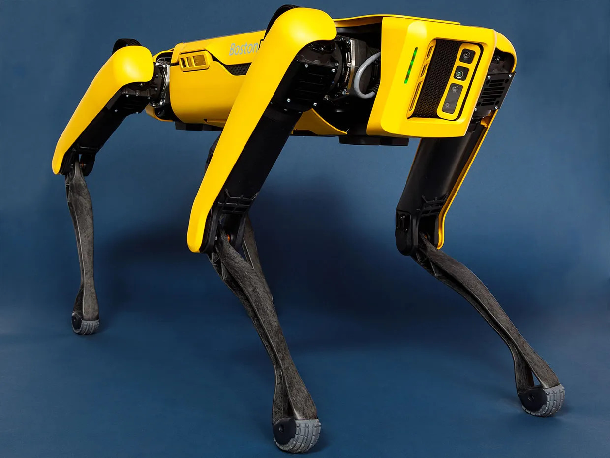
12 DOF - Spot by Boston Dynamics.
Image: IEEE Spectrum
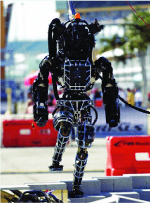
28 DOF - Atlas by Boston Dynamics.
Image: ResearchGate
The 12 DOFs of the Spot are a summation of 3 DOFs per leg, each DOF being the roll, pitch and yaw at the four joints. For the Atlas, the 28 DOFs consist of the neck, shoulder, elbow, wrist, waist, pelvis, knee and ankle joints.
Classical motion planners are highly dependent on the degrees of freedom of a robot due to the need to plan the control action for each degree of freedom separately. This is because each degree of freedom translates to a variable in the control space of the robot, which the planner needs to optimise. This makes a motion planner, which can plan efficiently in high-dimensional spaces, of the utmost importance.
To put things into perspective in Cartesian space: To plan the optimal path in a 10x10 2D grid, we need to calculate the relative cost to reach each of the 100 cells. Similarly, 1000 cells for a 10x10x10 3D grid. This means planning the x, y and z positions with only ten possible values each. However, in the real world, robots may have to optimise the controls for each of their motors for even 360 possible positions, or even more if we are operating on a sub-degree precision.
On the same note, sampling-based planners throw out the need for the planning domain to be discretized. In simple terms, for A*/Dijkstra’s algorithm to be implemented, a discretized version of the state space needs to be created. However, sampling-based planners are only limited by the precision limit of the computer, and thus are capable of planning in continuous space.
And finally, sampling-based motion planners come with the added benefit of customizability. One important component of a sampling-based planner is the steering function (the detailed description of which is not in the scope of this article). According to the physical dynamics of the robot being used, the steering function can be formulated to give the most precise path possible. For instance, the path needed for a human to move 1 metre to their right is not the same as the path required for a car to move 1 metre to its right, due to the sheer motion constraints of the vehicle. These types of limitations can be modelled into sampling-based planners.
3. How They Work
Traditional sampling-based motion planners work on the principle of rejection-based sampling. To make this easier to understand, let us take a simple robot.
Consider the map of your neighbourhood; this will be our obstacle map, which can be treated as an occupancy grid or graph in computational terms. In this example, we aim to plan a trajectory for a robot to drive from our house to the supermarket, say from our blue house on the top-right, to the orange supermarket on the top-left of the map.
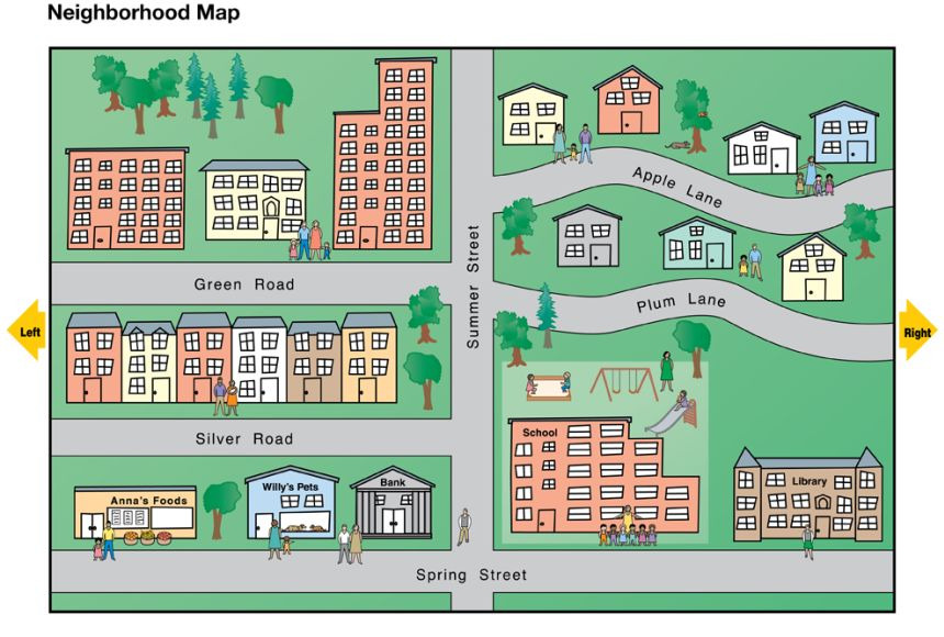
A Local Map. Image: National Geographic Society
A sampling-based planner would first randomly sample a point in the map. Say, it samples the coordinates of the community swimming pool. We know for a fact that the swimming pool is not a viable path for the robot, and so we reject it. The planner samples again and, this time, picks a point on a road somewhere on the map. This point seems reasonable, but is that road location reachable from our home? If not, try again, and if yes, voila! This is how rejection-based sampling works. The same is depicted in a sample obstacle map below (black obstacles; white unoccupied space) - 4 sampled points lie within obstacles and were hence rejected (red), after which one feasible point (green) was sampled.
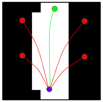
Schematic for rejection-based sampling
Using this clever strategy of sampling random points in the state-space (achievable states; locations in our example), sampling-based planners eliminate the need to calculate possible trajectories by traversing over each point. However, this comes at a cost. Traditional planners, although computationally expensive, assure the optimal solution. Sampling-based planners, however, are non-deterministic in nature, and the optimality of their solution is most often asymptotic. This means they will find a solution quite fast but converge to the optimal solution over time. This is especially true for RRT*, one of the most popular sampling-based planners, and this property is known as asymptotic optimality.
4. Different Variants
Over time, the robotics community has seen a lot of optimisation of the subparts of these planners and introduced variants tailored to solve specific use cases.
First introduced at Iowa State University by Steven M. LaValle, Rapidly-Exploring Random Trees or RRTs were a data structure with immense application in a wide-variety of motion planning problems. Utilising the benefits of randomised planning algorithms, RRTs especially made the task less painful for high-dimensional planning scenarios. Given a start and goal point in a known map, an RRT would sample a random point on the map. Then, using a user-defined function, the (Boolean) validity of the sampled point is checked. If the point is feasible (true), it’s added to the tree, otherwise it’s rejected and a new point is sampled.
Developed at MIT, the simplest asymptotically optimal planner is the RRT* - an improvement over the traditional RRT with rewiring of the tree over time. Let us break down these keyword features which the RRT* introduces on top of the RRT :-
- Asymptotically Optimal: An RRT planner finds a path if it exists. This does not guarantee the optimal path in any planning scenario. In case of an RRT, it is guaranteed that if a path exists, the RRT planner will find the optimal path asymptotically. This means that it will iteratively converge (if not perfectly determine) to the optimal path.
- Rewiring the RRT: The ‘star’ symbol or asterisk in RRT* refers to the rewiring feature introduced in the algorithm on top of the RRT idea. Rewiring is the process of deleting suboptimal edges of the RRT tree, to replace them with edges with lower cost. This process enables RRT* to be asymptotically optimal, and thus converge to the optimal solution iteratively. A detailed explanation of rewiring can be found in the resources below.
This variant is prevalent in the industry due to its ease of implementation and low computational cost.
Some useful resources to learn more about RRT and RRT*:-
- Sampling-based Optimal Planning : A Reading Group (YouTube)
- Robotic Path Planning : RRT and RRT* (Medium Article)
- AtsushiSakai/PythonRobotics : Python Implementations (GitHub)
- RRT, RRT* and Random Trees : A video guide by Aaron Becker (YouTube)
Another prevalent variant, which uses a hack to reduce the search-space, is the Informed-RRT* or the I-RRT*. This operates by mathematically constraining the search-space iteratively, depending on the current best-cost path found. Reducing the search-space helps reduce the computational cost significantly (which is analogous to not having to search for one’s toothbrush in the garage, thus saving time!). A comparative study on different sampling-based motion planners can be found in my repository.
Recently, the motion planning community has also experimented with the intersection of sampling-based planners and deep learning, giving rise to motion planning networks (MPNets), a giant leap forward in sampler variants. Extending this work, frameworks such as Dynamic MPNet and MPC-MPNet also add functionality for robust planning, by introducing a learnt sampling heuristic and thus making the sampler intelligent. These planners use a diverse set of sample worlds to train the sampler, and then detect similar features in their environment during deployment, to predict informed samples of possible waypoints.
5. Sampling-Based Planners in the Wild
Have you ever wondered how house robots work? The tiny ones which clean your homes while you’re at work, or mow your lawns during the day. Knowing the map of your house, these trivial robots use such motion planning algorithms to plan their trajectories in real time.
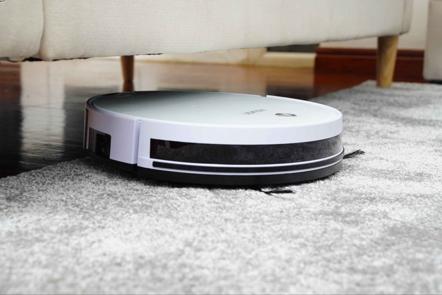
A Robot Cleaner. Image: Robots Science
And it’s not just for cleaning robots, RRTs have also been incorporated in software stacks to test out Mars exploration vehicles (article by NASA JPL), due to the sheer complexity of the control space. For instance, constraints such as calculating the shortest path, the path which would consume the least battery, etc. can be some constraints to employ while planning trajectories. The image below shows a sample trajectory for Spirit’s traversal across Martian terrain.
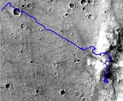
Schematic of planning for the Mars Exploration Rover. Source
Industrial automation relies heavily on the manipulation of objects, with tasks as trivial as segregation or pick-and-place operations. The control sequences for these operations cannot be hard-coded, so industrial manipulators have to plan their trajectories on the go to perform automation tasks.
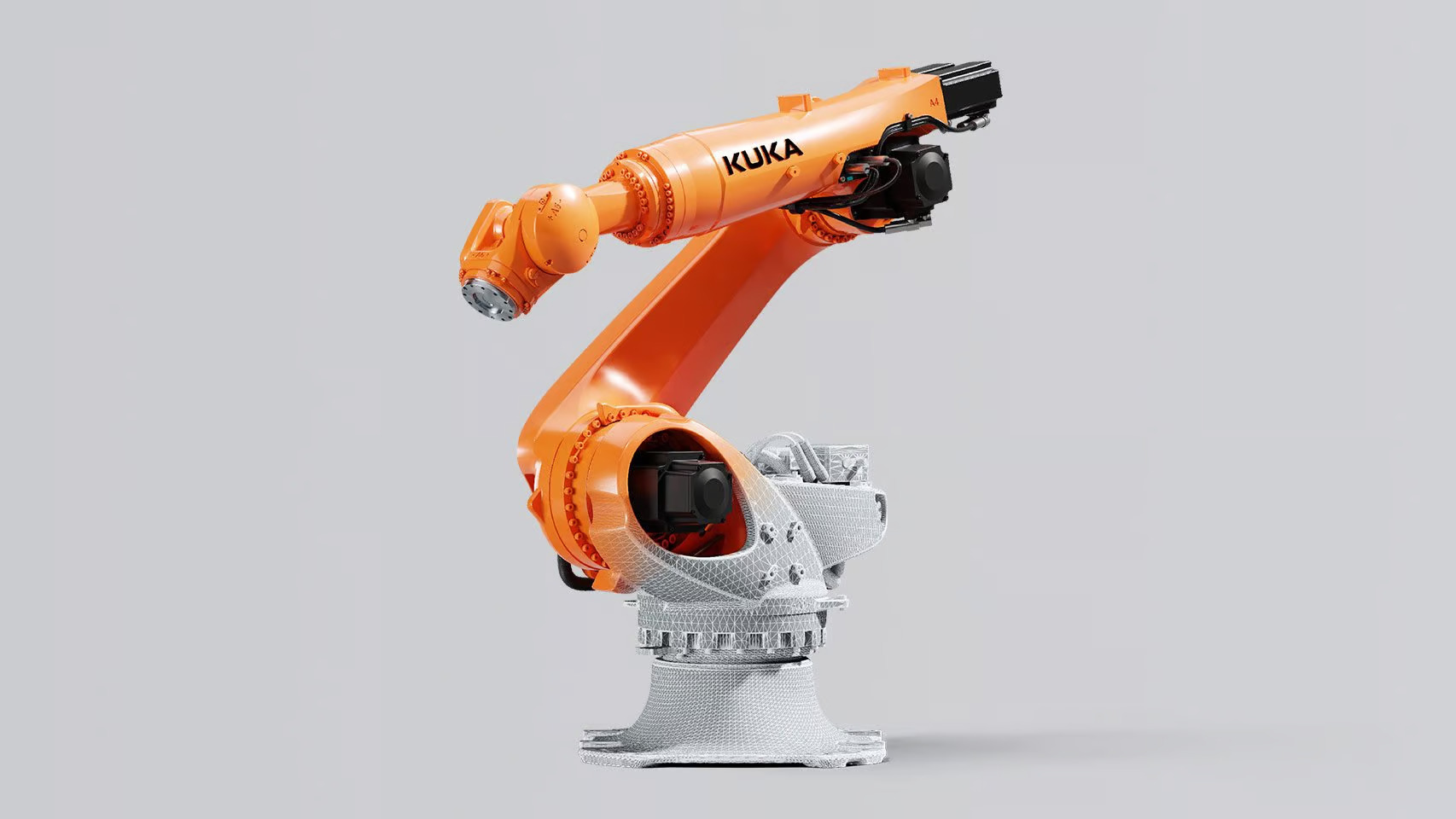
KUKA Industrial Manipulator. Image: KUKA Robotics
6. Conclusion
In this article, we started by understanding the need for sampling-based planners to solve this problem. Then we went into detail about the working of traditional sampling-based planners and rejection sampling. We then explored the different variants of sampling-based planners found in industry and academia and how they differ. And finally, we looked at some real-world (and out of this world) applications, and discussed the future of sampling-based planners.
This marvel of introducing scalability to motion planning frameworks was a great step towards planning for complex robots. The advent of sampling-based motion planners also opened doors to innovation in the different parts of the planner, such as the sampler, steering function, etc. The future of motion planning holds immense scope for improvement as new applications are found in space technology, domestic robots and industrial automation.
About the Author
Jaskaran Singh Sodhi is a senior undergraduate at IIT Kharagpur and incoming graduate robotics student at CMU, and has been working with robots for the past three years. He is passionate about autonomous racing and indoor navigation. He can be reached via email or LinkedIn.

